Automated Software Performance Monitoring for the ATLAS Experiment

Name	Douglas Lindsay
Organisations	CERN-HSF, Argonne National Laboratory, University of Washington
Mentors	Dr. Maciej Szymanski, Dr. Tatiana Ovsiannikova
Project	Automated Software Performance Monitoring for the ATLAS Experiment
Repository	atlaspmb/PerformanceMonitoring

Background

The ATLAS Experiment at CERN is immense in more ways than one; not only is it the largest particle detector ever constructed, but it also produces an enormous amount of data, exceeding 60 TB/s during active operation^[1]. Even after the Trigger filters this down to just a few gigabytes per second^[2] of interesting events, this volume of data was still large enough to warrant the development of the ATLAS Data Processing Chain, a massive software pipeline that turns this raw data into physics-ready datasets. The Data Processing Chain is comprised of a number of steps which are further divided into small units called jobs, each of which is processed by hundreds of computing clusters all around the globe using the Athena software framework, a huge codebase containing about 4M lines of C++ and 1.5M lines of Python^[3]. Since each job uses a subset of Athena’s 27,000 components (small and reusable software modules performing a specific function), the performance of each component impacts the performance of the Athena framework as a whole.

Figure 1: Steps in the ATLAS Data Processing Chain

Motivation

Therefore, it’s immensely important to monitor the performance of all of these components and ensure that they remain performant and resource-efficient. Over the course of Google Summer of Code, I collaborated with the ATLAS Software Performance Optimisation Team (SPOT), which tracks numerous job-level and component-level metrics (e.g. RAM usage, CPU time, etc) between nightly builds of Athena using the ATLAS Performance Monitoring Board (PMB), and reports anomalies therein. However, the definition of an anomaly is fuzzy at best, and to complicate matters further, many metrics are noisy, have missing data, or exhibit frequent one-nightly-build regressions due to configuration issues, quickly remedied bugs and more. For example:

• A component-level metric suddenly worsens between nightly builds, degrading the performance of all jobs using that component.
• A job-level metric suddenly improves between nightly builds. Although this may just mean a component was optimised, it may also mean a bug was introduced.

Figure 2: The anatomy of an example metric, and a process by which a SPOT member might identify anomalies therein.

With dozens of jobs using tens of thousands of components, and dozens of metrics for each, this is just too much data for any human to analyse by hand, so an automated solution was needed. This is where I came in: incorporating an anomaly-detection step into the existing SPOT performance monitoring pipeline which uses statistical and machine-learning techniques to detect, report and diagnose these anomalies, and issue alerts when appropriate.

Introductory projects: Screening task and OpenSearch exporter

Before I started on anomaly detection, I first familiarised myself with the codebase through two smaller projects.

The first of these projects was my initial screening task as part of the GSoC selection process, where I used prmon, a HSF performance monitoring tool, to record the performance of a simulated process and identify anomalies in various metrics therein, such as PSS (proportional set size), wall time and more. This both introduced me to the metrics that I would be analysing over the subsequent weeks and to a number of statistical and machine-learning techniques (some of which were more effective than others) that would form the foundation for the later algorithms I would design in the GSoC project. For brevity, further detail is omitted here but a write-up for the screening task can be found on my GitHub.

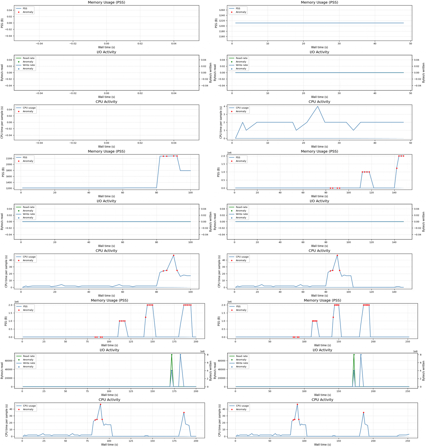
Figure 3: Real-time monitoring of prmon output and classification of anomalies.

After being accepted to GSoC, I familiarised myself with the SPOT pipeline via a smaller project: adding a step to the pipeline that would export the computed metrics to OpenSearch (a search and analytics suite used to explore large volumes of data in real time), as part of a broader migration within SPOT from locally stored SQLite databases to cloud-based records with a view to eventually replacing the Performance Monitoring Board with Grafana dashboards. This was a fairly simple project, but it was still useful for setting up my local environment, learning the database structure, and understanding the distinction between job-level, stage-level, domain-level and component-level metrics. This also set some of the groundwork for the main project, since OpenSearch includes some level of anomaly detection and alerting using a Random Cut Forest, an algorithm that I would later explore in considerable detail.

For purposes of efficiency, the script only uploaded the metrics for the most recent nightly build. In the closing weeks of the project, I returned to the OpenSearch exporter and augmented this functionality by adding an additional command-line flag that allowed the script to ingest a merged database (i.e. containing metrics from many nightly builds, not just one) and upload the entire history contained within that merged database. This meant that the script could now be used not just to manually upload the entire history of all the existing SPOT databases, but also as part of the PerformanceMonitoring pipeline to upload the metrics for just the most recent night, as previously.

The GSoC project: Performance monitoring

Metrics

Once I was familiar with the SPOT codebase, I embarked on the main project, beginning by exploring the process by which the metrics displayed on the Performance Monitoring Board were generated. It turned out that these metrics were very tightly coupled to the script that produced their plots, create_spot_plots.py, so I initially opted to re-implement this logic within the anomaly-detection script (detect_anomalies.py) I developed. However, due to the number of distinct metrics and edge cases in the implementation therein, it quickly became apparent that this would be much more effort than just refactoring the codebase to encapsulate the metric-generation logic in its own script, generate_spot_data.py, which produced metrics that could be ingested by either the anomaly-detection or plot-generation scripts, or any other future scripts.

Autonomous anomaly detection

With the metrics obtained, I moved to developing a number of anomaly-detection algorithms and backtesting these on historical data to determine their effectiveness. These included:

• Bollinger Bands, a statistical technique widely used in financial modelling to identify outliers in univariate (one metric) time-series data using a moving windowed mean and moving windowed standard deviation to compute z-scores and flag points with scores exceeding some threshold.
• Exponentially weighted moving averages (EWMA), which are similar to Bollinger Bands except that the mean and standard deviation are computed using an exponential falloff rather than a window.
• Isolation Forest, a multivariate machine-learning technique for identifying outliers in multidimensional data (i.e. multiple metrics at once).
• Random Cut Forest, a similar multivariate technique that is slightly more efficient and works on online data.
• Z-space distances, a simple multivariate technique which maps data points to z-score space with position on each axis corresponding to one metric and identifies outliers therein based on the Z-score of their distance from the origin.

When backtested on historical data, neither Isolation Forest nor Random Cut Forest proved to be effective for identifying the kind of multi-day step-change anomalies observed in SPOT data, particularly due to their inability to detect a regression to a performance level that was similar to a past performance level. While they were effective at detecting 1-day regressions, they were much less effective at detecting persistent regressions (the kind of anomalies that SPOT is interested in), were much more computationally expensive than Z-space distances, and did not handle data where either the anomalies or the normal data were at the extreme ends of the observed range (extremely common in SPOT data, and a phenomenon I first identified as early as the screening task). Taking all this into account, I opted to use the simple and robust Z-space distances as the only multivariate detector in the final program.

Of the two univariate algorithms (EWMA and Bollinger Bands), I found that EWMA overweighted more recent results and therefore ran the risk of absorbing small changes without reporting an anomaly. As such, I opted to avoid it and instead modify the Bollinger Bands approach to produce two algorithms, one operating on the metrics directly and one operating on their first derivative.

Figure 8: A one-day regression versus a multi-day regression. When these regressions occur, they look exactly the same. But one’s anomalous, and one isn’t. How do we tell them apart?

As shown in Figure 9, these were very effective at detecting deviations from normal performance, but were incapable of distinguishing between normal one-day regressions and anomalous persistent regressions, a problem I resolved by making both detectors wait a few days to confirm that a regression was persistent before reporting it (an anomalous persistent regression looks like a step change in a metric and therefore an impulse in its first derivative, so the two detectors identify the same phenomenon and are more likely to catch a false negative produced by the other), which is shown in Figure 10. I employed both the direct-metric and first-derivative univariate detectors in the final program.

All three detectors operated independently of each other.

In my backtesting, I found that aside from a few days where system configuration changes (e.g. a migration to a new test machine) led to anomalies across a large number of metrics, most metrics were relatively stable with no anomalies at all. I therefore tuned the anomaly detection parameters to be rather strict to prevent an excess of false positives. Broadly speaking, there were three classes of tunable parameters:

• Z-score thresholds: For all three detectors, a point will not be reported as an anomaly if the magnitude of its’ Z-score is less than some (detector-specific) threshold. An appropriate Z-score was therefore be selected in line with the approximate number of anomalies in the data to provide a good trade-off between false positives and false negatives.
• Minimum percentage changes: Some metrics are very stable with an extremely small amount of noise, but a detector operating purely on z-scores may still report anomalies even though the relative change was negligible, so I instituted a minimum percentage change for a regression to qualify as an anomaly, reducing false positive rates. As the number of false positives was overall reduced by this change, I could also decrease the Z-score threshold slightly, reducing the false negative rate.
• Confirmation period: Each detector waits for a short period after a regression to confirm that it is persistent and not transient/noise. By virtue of reducing the false-positive rate, this also eliminates a great deal of noise-based variations, meaning that the previous two thresholds can be decreased, reducing the false-negative rate.

The advantage of having three measures was that, as noted above, this provided a much greater degree of resilience against false positives and negatives, as each measure did not need to be especially strict.

Autonomous anomaly reporting

To inform the SPOT team about anomalies, I implemented a simple alerting system using a webhook on Mattermost, the primary communication platform used by SPOT. This reports salient characteristics of each anomaly such as the z-score and percentage change in an easily skimmable and digestible form, as well as providing various sources of additional information, such as the TrigMR and GitLab Athena nightly build merge request summary pages.

Figure 11: An example Mattermost message reporting anomalies, including some metadata about the job and each anomaly found in metrics therein.

Additionally, I modified the script that creates the plots on the ATLAS Performance Monitoring Board so that it invoked my anomaly-detection script and included the detected anomalies on the plots for the PMB.

Autonomous anomaly diagnosis

The last major piece of functionality I implemented was a routine that would attempt to connect job-level anomalies to their candidate root causes in the form of component-level anomalies, meaning that a high-level performance regression could have its source identified and resolved faster. For example, a job-level anomaly and a candidate component-level anomaly that potentially caused the job-level anomaly will typically have the same sign (except in the cpu edge case detailed below), allowing the root causes to be narrowed down. Job-level anomalies can be divided into three classes, and I implemented a distinct approach for each:

• Container size (sizeperevt): For a job-level anomaly in this class, the root-cause detection attempts to identify any domains of that job that themselves contain anomalies, and then any component-level anomalies (candidate root causes for the job-level anomaly) within those domains.
• Memory (malloc): For a job-level anomaly of this type, the root-cause detection attempts to determine what stage (Initialize, First Event, Execute, Finalize and preLoadProxy) a component-level anomaly might be found in using the stage the job-level anomaly was found in; if it did so successfully it filters component-level anomalies to only those within that stage.
• CPU (cpu): For this class of anomaly, the same procedure is followed as for sizeperevt, except it accounts for the fact that certain job-level metrics with units 1/s are inversely correlated with the component-level metrics, which are generally in units s.

While this is imperfect, it is still a useful tool for narrowing down which components are responsible for observed regressions.

Finishing touches

With the anomaly detection software essentially complete, the final weeks of the project were predominantly spent polishing it to produce the highest-quality result possible:

• Implementing a clean and concise CLI for each of the scripts
• Writing documentation for how the scripts should be used (e.g. --help messages)
• Typehinting all my software until it satisfied Pylance on Strict mode, and ensuring no partially-unknown types from external libraries like pandas or matplotlib were exposed.
• Incorporating my anomaly-detection script into the bash scripts comprising the performance monitoring pipeline
• Addressing various edge cases:
  • Anomalies may occur in VMEM/PSS which are job-level malloc metrics but cannot be narrowed down to a specific stage: Resolved by not filtering by stage in this case.
  • Historical nightly build timestamps in merged databases do not have a 1:1 correspondence with dates, because sometimes the pipeline fails and data is lost: Resolved by operating entirely in terms of nightlies with an associated date, rather than the other way around.
  • Some metrics had a different name every day, causing data loss: Temporarily hardcoded an exception for these metrics and notified the team responsible and then, when this was resolved, removed that exception.
  • Empty Mattermost reports would be produced if no anomalies were found: Resolved by not producing a report in these cases.
• Tuning parameters, e.g. the minimum standard deviation and minimum percentage change for a regression to be reported as anomalous, to improve accuracy further.

Outcomes

The primary outcome of my project was three merge requests to the PerformanceMonitoring repository, totalling a combined ~3600 lines of code changed.

• atlaspmb/PerformanceMonitoring!38: The original merge request for the script for uploading all metrics from the most recent nightly build to OpenSearch as part of the existing performance monitoring pipeline
• atlaspmb/PerformanceMonitoring!39: Refactors the metric-generation logic to its own file, and includes the anomaly detection, reporting and diagnosis software.
• atlaspmb/PerformanceMonitoring!40: Adds a standalone mode to the OpenSearch exporter script that permits it to be manually invoked on a merged database (i.e. one containing metrics from multiple nightly builds) to upload all that history at once.

Together, these make it possible for the SPOT team to identify and fix regressions more quickly than was previously possible through manual inspection.

Further work

Although the anomaly detection pipeline is complete, as with any software project there are areas that could be explored further:

• Implement a missing-data detector, because step-change regressions, which the Bollinger-based univariate detectors pick up, are not necessarily the only kind of anomaly - for example, a bug could cause a crash with no data being reported at all, leading to missing data. I experimented with a missing-data detector but ultimately did not prioritise implementing this.
• The ability to locate the corresponding repository for any components with anomalies would be very useful.
• The orchestration scripts could be migrated from Bash to Python modules so the entire SPOT codebase is in one language and is easier to read and debug.

Final reflection

Google Summer of Code 2026 was an incredible program, especially with CERN-HSF. Working on high-energy physics at CERN has been a lifelong dream of mine, and having the opportunity to collaborate in an adjacent area before even completing my undergraduate degree and despite living in a non-Member State is incredible. Only two years ago, I traveled to Switzerland solely to tour CERN, and it feels surreal that code I’ve written will now be aiding in the operation of the very detector whose control room I visited such a short time ago. I can’t wait to see where this path leads, and I’m immensely grateful to both Google and CERN-HSF for making this possible.

On the more technical side, working on a production-grade HEP codebase was a fantastic opportunity to develop my skills in software development. Although it was challenging at times, I’ve learnt an enormous amount about performance optimisation, software architecture and industry best practices. Maciej and Tatiana’s mentorship and guidance was invaluable, and I’d like to thank them both personally since this project wouldn’t have been possible without them.

AI Usage

AI was used to a limited extent in this project, principally for research and low-level implementation details. Although I experimented with a number of different models, a common thread was that they were unfamiliar with HEP and would often make incorrect assumptions implicitly, meaning that in most cases reviewing and unit-testing AI-written code was more effort than just writing it myself. I also found most AI models had a strong tendency to produce “spaghetti code” without thought for long-term architecture or maintenance, although stronger models were somewhat more resilient to this.

References

^[1] ATLAS Experiment at CERN: Trigger and Data Acquisition

^[2] Vazquez, W.P. on behalf of the ATLAS Collaboration: The ATLAS Data Acquisition System in LHC Run 2

^[3] Mete, A.S., Nowak, M., and van Gemmeren, P. on behalf of the ATLAS Computing Activity: Persistifying the complex event data model of the ATLAS Experiment in RNTuple